ECE565 Nodule Detection based on Statistical Signal Analysis (Spring2015)

This is a course project I have done by myself for course ECE565, Computer Vision and Image Processing. The lab requirement asks us to develop a method to detect nodule candidates in a medical image of lungs using the algorithms that we have learned from the class. I put together a bunch of image preprocessing methods and acquire a few features from each nodule candidate. Then I manually selected an area in feature space using human experience and marked every candidate in this area as suspicious nodules. If I have enough data sets, I should able to train a simple SVM to characterize the nodules from the feature space I created. Furthermore, If I have more data, I will prefer to build a YOLO similar convolutional neural network to detect and locate the position of the nodule in a CT scan.

Table of Contents

• ECE565 Nodule Detection based on Statistical Signal Analysis (Spring2015)

  • Introduction

  • Methods and Results

  • Discussion and Conclusion

  • References

Introduction

This project presents a method based on computer vision to detect the nodules in a series of Computed Tomography (CT) images; it is a computer-aided detection system for lung nodules in chest CT images. The algorithm contains different image processing techniques including image segmentation, labeling, filtering, etc. The potential candidates of the nodules will be marked in the original image. The processed image can be shown to the doctor for further evaluation; or it can build the 3D lung module for a better diagnosis. The algorithm is implemented in MATLAB. In Figure 1 is the original CT images to be processed, the nodules are labeled by white boxes.

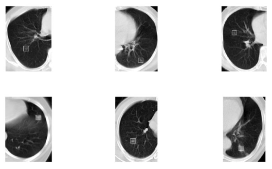
Figure 1, Original Chest CT scans with nodule circled

Methods and Results

There are mainly four steps in order to accomplish the lesion detection system.

• Firstly, the lung will be recognized as an object and be separated from the background in the image.

• Secondly, from the separated lung in each CT scan, several lesion candidates will be detected.

• Thirdly, the different lesion candidates will be labeled, and the algorithm’s features will be calculated.

• Lastly, by using the features of different candidates, possible candidates are selected and marked in the original CT scans. In the following subsections, the details of the algorithm in these four steps will be presented.

Step 1: Segmentation of the lungs

The segmentation of the lungs is performed by using the strategy of threshold and morphology filtering. By drawing the original CT scan histogram shown in Figure2, we can know that each CT scan consists of two parts, object and background. Both of them generally obey the Gaussian distribution. By observing the original image, the object in the image is the dark part; the background is brighter than the object. The prime of separating these two sections is to find a threshold and remove the pixels that have a higher value than the threshold. I wrote two functions to calculate the threshold. The first method is by using iterative segmentation, which is the one presented in the class. The second method is OTSU algorithm.

Figure 2, Histograms of the original CT scans

There is no big difference among thresholds that are calculated by using different methods. The result of the segmented image can be shown in Figure 3. By observing the segmented lung, it can be easily found that the lungs are incomplete, there are some holes on it and the edge is not smooth. So we need a morphology filter to adjust the shape of the segmented image.

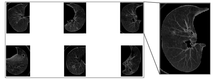
Figure 3, Raw object segmentation

The morphology filter is implemented by applying erosion, dilation, and hole filling algorithms to the original image. First, the raw object will be converted from a gray level image to a logical image with only two values to represent each pixel; the logical image is called the mask of the object. After so, an expansion operation will be applied to the mask image. After the expansion, erosion will be applied to the expanded image. After these two steps of operations, the edge can be smoother and most of the small holes in the object are filled. However, some big holes are still not completely filled; we will use image fill operation to fill the whole in the image. After the morphology filtering, we will obtain an object mask. The object can be easily selected by combining the original image and the object mask, as shown in Figure 4.

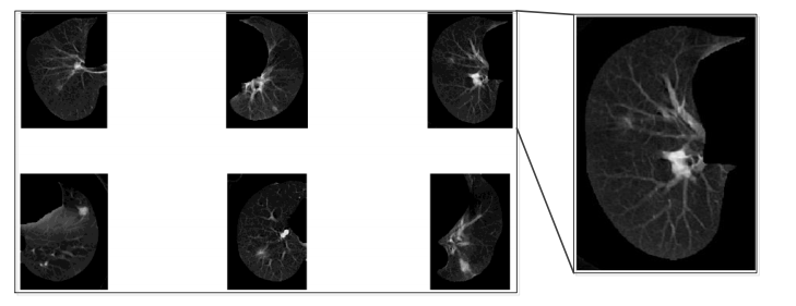
Figure 4, Final object segmentation

The potential problem of using the threshold and morphology filtering to obtain the object of the image is that, it may misclassify the tissue in the corner as the object. What’s more, the erosion and expansion operation may change the shape of the object. It is more like an estimation of the shape of the object, not precisely. However, as we can see in Figure 4, the performance of this algorithm is very nice.

Step 2: Detection and segmentation of lesion candidates

The detection and segmentation of the lesion candidates can be done by using threshold based segmentation. The prime is how to find the best threshold in the object that we obtained from step one. This threshold can be decided by using a constant summarized from the experiments. However, this method doesn’t have a good performance. In order to find a better way to find the threshold, I plot the histogram of the segmented object. Figure 5 shows the histogram of the object image.

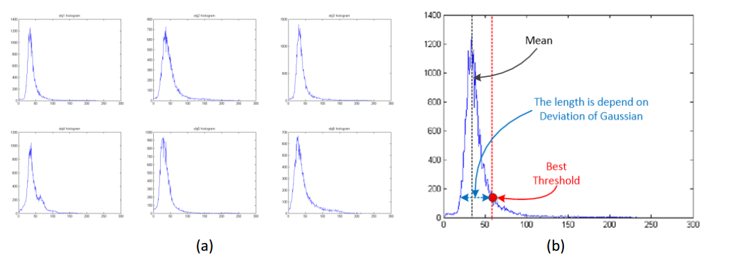
Figure 5, (a) Histogram of the object image, (b) Threshold selecting strategy

As we can see in Figure 5 (a), the object generally obeys the Gaussian distribution. For a Gaussian distribution, there are two parameters, mean and deviation. Take a closer look at the object histogram, Figure 5 (b) shows the way I am using to find the threshold. In Figure 5 (b), the mean value can be easily found by locating the maximum value in the histogram. The deviation of the Gaussian function is found by using the MATLAB function ‘std’. After trying the threshold with different values, I found that the best threshold is always at the position of the red dot in Figure 5 (b). By using the mean and deviation of the Gaussian distribution, we can calculate the best threshold by using the following equation.

\(\mathrm{T}_{-} \text { best }=\mathrm{a}^{*} \mathrm{avg}+\mathrm{b} * \mathrm{dev}+\mathrm{c}\).

In the equation, a, b and c are the experience coefficients for fixing the position of the best threshold. Table 1 shows the deviation, mean, and best threshold. The experience coefficients are: a=1.1, b=0.025, c=-4. After using the selected threshold to segment the object, we will obtain the raw nodule candidate in Figure 6.

Table 1 Histogram mean, deviation, and best threshold

Figure 6, Raw nodule candidates after segmentation

As we can see in Figure 6, there are many small dots existing there as a noise. Indeed, we can take all these dots as nodule candidates. By using the classification technique, these dots can be easily eliminated because of the size. However, it will take extra time to eliminate in the step 4 than just eliminate the small pepper like dots by using median filter. After the median filter, the nodule candidate can be shown in the figure 7.

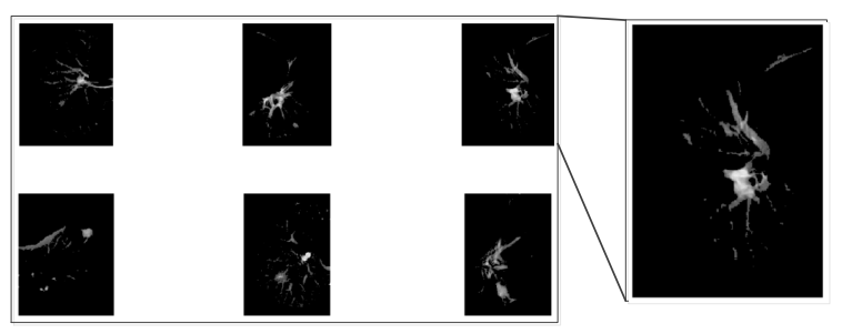
Figure 7, Nodule candidates after median filter

My algorithm’s potential problem is that the histogram of the object image is not smooth; the average calculation function finds the value by using the maximum value in the histogram. It recognizes it as a peak, and then the average value is located by the maximum value. When the signal is noisy, the peak value may not appear at the average location precisely. And the equation is an experience equation, which will need manual adjustment for the value of a, b, and c.

Step 3: Connectivity analysis and feature extraction from the segmented lesion candidates

In this step, the nodule candidates will be separated by using a connected area labeling strategy; the features of these candidates will be calculated and saved to do the feature selection in step 4. Before doing the connected region labeling, the gray level image will be converted to a logical image. Figure 8 shows the nodule candidates image after converted to logical image. With the build-in function ‘bwlabel’ in the MATLAB image processing toolbox, the connected region of the image will be labelled with the same number. After the image labeling, different nodule candidates in the image will be labelled in different numbers. For each image, we have a list of nodules. Each nodule will contain two feature information, they are circumference and area. These two features will be used to eliminate the fake candidates.

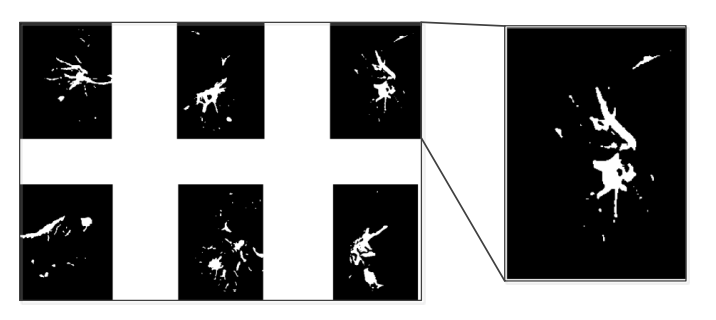
Figure 8, Nodule Candidates in a logical image

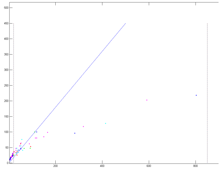
Figure 9, Feature of nodule candidates in the same image

In Figure 9, X-axis is the area of candidate; Y-axis is the circumference of the candidate. Candidates in different scan will be colored in different color. This image will be used in step 4 o do feature selection and classification. The issues associated with feature extraction are that the circumference calculation is done by using the Laplacian filter to find the edge of the candidates. However, the Laplacian filter may change the shape of the candidates; this will make the circumference not accurate.

Step 4: Feature selection and classification of the lesion candidates by using a rule based scheme

From Step 3, we obtained the image with all the nodules segmented and labeled. The information of different nodule candidates is extracted from the nodule. The rest of the work is to eliminate those candidates that are obviously not a nodule. First of all, those candidates with a very large size or very small size, they are not nodules. For the candidates with very small size, it is just a noise in the image. For the candidates with a very large size, it is the trachea or vessel in the lung. What’s more, the line structures in a lung CT image are the trachea or vessel. In order to eliminate the line structures in the image, the ratio of the circumference and area will be calculated. The area is calculated by counting the pixels in the target candidate. The circumference is calculated in the same way; the difference is that an additional Laplacian filter will be applied to the nodule candidate. Laplacian filter will show the edges of the target block. Count the pixels after the Laplacian filter will give us the circumference of the target candidate. The ratio of circumference and area can tell the approximate structure of the target candidate. For the candidates with a fat shape, the ratio will be small. For the candidates with a thin shape like a line, the ratio will be large. Figure 10 is a 2D feature space. The red dash line is the restriction of the ratio between circumference and area. The coefficient 0.9 is an experience parameter. When the ratio is smaller than 0.9, I will recognize the candidate as a line structure, and it will be eliminated in the final result. The blue lines are the minimum size of the candidate and the maximum size of the candidate. Only the candidates that located in the blue area will be recognized as a final nodule candidate. Figure 11 shows the nodule candidates after filter the small candidates away.

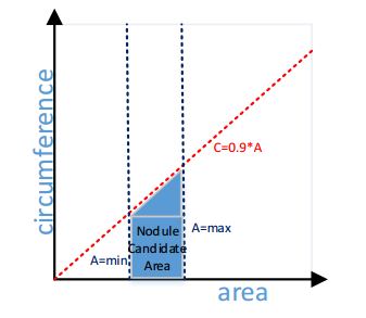
Figure 10, 2D Feature space

Figure 12 shows the nodule candidates after filter the large candidates and line like candidates away. It is the final result of nodule candidates. In order to clearly show the selected nodules to the doctor, additional operations will be implemented to circle the nodule in the original image. First, the image expansion will be used again to make the nodule candidates larger. Then a Laplacian filter will be applied to the expanded nodule candidates to obtain the edges of the original image. The edges detected from the nodule candidate will be used as a mask to show the nodules in the original CT images as it is shown in Figure 13.

The performance of accuracy can be calculated by using the ratio of the number of real nodule and the number of nodule candidates. The performance of speed can be calculated by the running time counted by MATLAB. The running time is a little bit tricky. When I run the code directly, it will cost less than 1 sec, however, when I run it and count the time, it will take 5.426 sec. Table 2 shows the accuracy performance of my algorithm.

As for the issues in my algorithm, my method of eliminating the fake candidates is a linear method. I set a certain range of the features, and remove the entire candidate with features out of this area. Some more advanced techniques can be used to eliminate the fake candidates and it can give us better result. The advantages of rule based scheme are that it is simple to implement and understand. The problem is that the accuracy of the algorithm is not as good as some other methods.

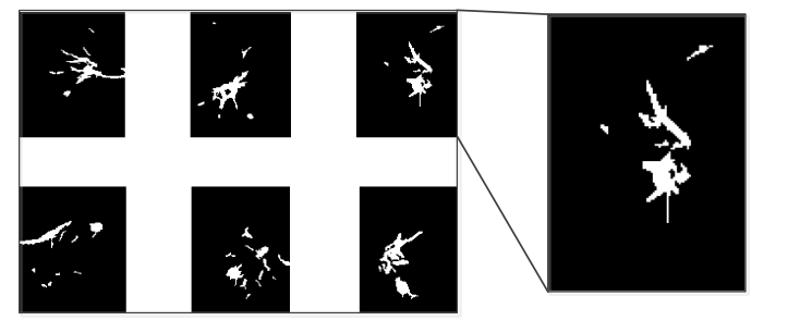
Figure 11, Nodule Candidate after Filter away the Small Elements

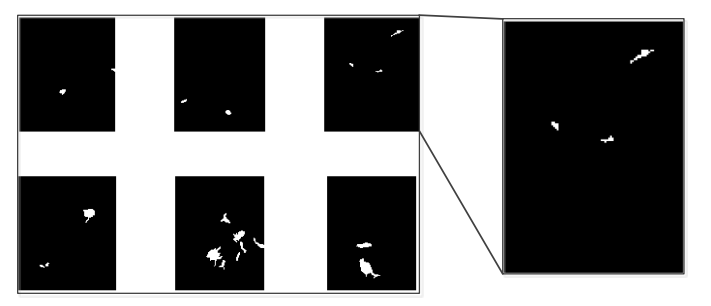
Figure 12, Nodule Candidate after Filter away the Line Structure and Huge Elements

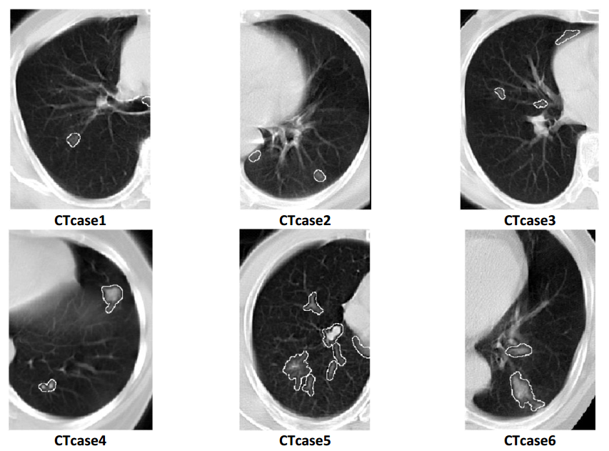
Figure 13, Final Result of Nodule Candidates

Table 2 Accuracy Performance of the Nodule Detection Algorithm

Discussion and Conclusion

In this project we are asked to develop an algorithm to detect the nodules in a CT image by using the basic computer vision knowledge. The method I am using in the project incldue threshold finding, image segmentation, image spatial domain filtering, morphology filtering, etc. It helps me to understand what we have learned in the class and shows us the capability of computer vision in the real applications. The algorithm uses some basic image processing technique and most of the coefficients are manually set by the experiment. This will make this algorithm specialized for the certain series of image. To improve this and make the program stronger, the coefficients can vary with the input image. The result of this project can be used to further develop the3D reconstruction of the lung nodules.

References

1. Rafael C. Gonzalez and Richard E. Woods. Digital Image Processing (3rd Edition). Prentice-Hall, Inc., Upper Saddle River, NJ, USA, 2006. ISBN 013168728X.

2. N. Otsu. A threshold selection method from gray-level histograms. IEEE Transactions on Systems, Man, and Cybernetics, 9(1):62–66, Jan 1979. doi:10.1109/TSMC.1979.4310076.

3. Jean Serra. Image Analysis and Mathematical Morphology. Academic Press, Inc., Orlando, FL, USA, 1983. ISBN 0126372403.

4. Samuel G. Armato III, Maryellen L. Giger, and Heber MacMahon. Automated detection of lung nodules in ct scans: preliminary results. Medical Physics, 28(8):1552–1561, 2001. doi:10.1118/1.1387272.

Statement

This is a course project, all the raw data are provided by Dr. Kenji Suzuki through course ECE565 at IIT. Please contact me if you find any problem.