ECE584 DCT Implementation Optimization on VLSI level (Spring2014)¶

ECE584 is a course at IIT called VLSI Architecture for Signal Processing and Communication Systems. It is one of the best course I have took at IIT. The course teaches how to design and optimize signal processing algorithms on Hardware. This is the final project of EC584 in the semester I took this course. In the project, we are asked to implement and optimize a Discrete Cosine Transform (DCT) in HDL language. Me and another classmate of mine are teaming up in this project.

Table of Contents

ECE584 DCT Implementation Optimization on VLSI level (Spring2014)

Introduction ¶

In the project, two different methods will be applied to implement the 8-point DCT. One is direct implementation with algorithm reduction, another one is binDCT algorithm. The specific algorithm of these two implementations will be introduced later.

For that the DCT is with constant parameters, no adaptive algorithm is used, we can simplify the multipliers to some shifters and adders. This saves us a lot of hardware and can reduce the delay. In the whole process, we will use signed numbers. Specific signed adder is developed to meet the requirement which will be introduced later. The input will be 8 bit number and output will also be 8 bit number. The input will be extended to 12 bit immediately in order to assure that there will be no overflow in the computation. At the last stage, the output will be cut and only 8 bit will be reserved.

For the binDCT implementation method, after the implementation, the power, area and delay parameters will be measured from the ISE. These parameters can shows us the properties of these two implementations. At last, these two techniques will be compared to draw a final conclusion.

Background ¶

DCT is the abbreviation for Discrete Cosine Transform; it can transform the signal from time domain to cosine domain. It can represent a given signal in term of a sum of cosine functions oscillating at different frequencies. It is a powerful tool for signal analysis and can be applied to many important applications like data compression and so on. A DCT is a Fourier related transform similar to the Discrete Fourier Transform, but using only real numbers.

IDCT is the invert process of DCT; it can recover the original signal from the transformed signal. DCT and IDCT can be represented by the following equations.

\(X(k)=e(k) \sum_{n=0}^{N-1} x(n) \cos \left[\frac{(2 n+1) k \pi}{2 N}\right], k=0,1 \ldots, N-1\)

\(x(n)=\frac{2}{N} \sum_{k=0}^{N-1} e(k) X(k) \cos \left[\frac{(2 n+1) k \pi}{2 N}\right], n=0,1, \ldots, N-1\)

X[k] is known as the N-point DCT of the sequence x[n]. In our case N is 8. Two methods including direct implementation with algorithm reduction and binDCT algorithm will be used to implement the DCT transform. We will not implement the IDCT process and use MATLAB IDCT function to recover the transformed signal.

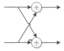
The original DCT process can be shown by using the DFG in FIG 1.

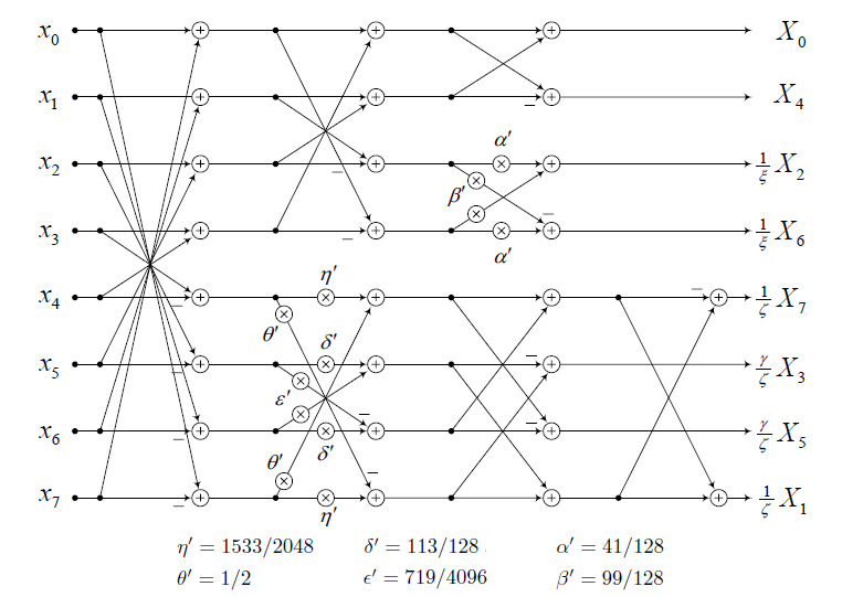
Figure 1, DFG of DCT¶

As we can see, 24 adders and 12 multipliers will be used in the implementation. In the following two sectors, it shows two improvement implementations based on this DCT structure. These two implementations have better performance compared to this one. Our task is to compare the performance of these two implementations.

Implementation ¶

DCT direct implementation with Algorithm Strength Reduction¶

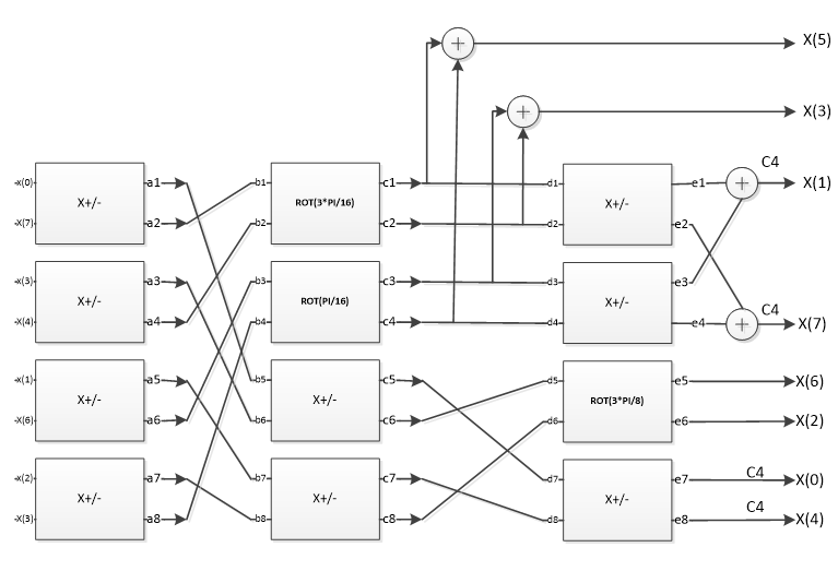
Figure 2 DCT Block diagram¶

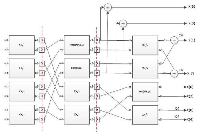
Figure 3 DCT Block diagram with Pipeline¶

binDCT multiplier-less DCT implementation¶

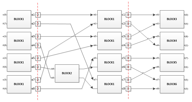
Figure 4, binDCT Blockdiagram with Pipeline¶

Block 1 only uses addition operation. It uses the Signed Adder mentioned before. It can handle the addition or subtraction of two real numbers. For subtraction, there is the need to change the subtractor’s sign bit before using Signed Adder.

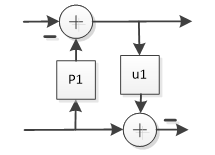
The design of Block2-Block6 follows the similar idea. The shift operation replaces multiplication because C5 parameters can be realized by the additions and subtractions of 2n. Take Block4 for example. P1= U1=3/8, which can be implemented as 2-1+2-2. Hence, in VHDL design, x*p1 can be realized as (x>>1)+(x>>2), which can be implemented as two shifts and one add operation. Hence, outa=(inb>>1+inb>>2)-ina, outb=inb-(outa>>1+outa>>2). In the code, shifts operations are realized as shift1.vhdl, shift2.vhdl, shift3.vhdl,shift4.vhdl, shift5.vhdl,… This can reduce the multiplication to shifts and subtraction operation. In addition, the signed addition can be implemented by using the Signed Adder block. Similarly, subtraction can be realized by negating the subtractor’s signed bit. All the blocks from block2 to block6 are the combination of shifters and adders. Compared with the original design, block2- block6 cost less, but they cannot generate accurate results, it is the estimation.

Functional Validation and verification ¶

Hardware description language VHDL is chosen to program the DCT. We use ISE from XILINX to synthesis and implement the design. In the ISE, it has a simulation tool called ISIM. I will use this tool to simulate the design and view the final result. If we use the ISIM, the test-bench is not necessary. But this is fit for the design with fewer inputs. In our design, 8 inputs are required. If we don’t have a test bench, input the numbers manually will lead to a heavy work. So I wrote a test bench with TESTIO package in VHDL. The read and write function in the TESTIO allows us to read the input from the .txt file automatically. After the simulation a new .txt file with output will be built to the destiny location.

MATLAB ISE co-simulation ¶

At the simulation phase, we will use MATLAB ISE co-simulation. The input can be generated by MATLAB and wrote to a stimuli.txt file. After the processing in ISE, response.txt will be created. By using MATLAB, we can analysis the result better. The simulation process will be listed below.

Creating the stimuli.txt file by using the MATLAB. The numbers in the stimuli.txt will be separated into several sets of data. Each set of data consists of 8 numbers. I wrote an m-function called stimuli_gen.m in MATLAB. This code can be found in the APPENDIX

Run the simulation in ISE and run the test bench in ISIM. The stimuli.txt will be read and converted to binary numbers and then be input to the DCT. After the output is generated, the test bench will again convert the binary outputs to decimal number and then write them to the response.txt at a specific location. The code of the test-bench can be found in APPENDIX.

Using MATLAB to read the response.txt to obtain the raw output data. The original data is coded as signed numbers. So the raw data needs to be processed before plotting. The convert function in the TESTIO can only convert the unsigned number. For example, the original data is -10, it will be 10001010. The converted number will be 138. I wrote an m-function in MATLAB to restore the original data from the raw data. The method is very simple; when the number is below 128, just keep it. When the number is over 128, I will subtract it from 128. After the conversion, the data will be stored in the matrix and plotted.

The last thing is to do the IDCT to the transformed signal with MATLAB IDCT m-function. This is to prove the correctness of the transform.

The whole process can be shown by the following flow chart.

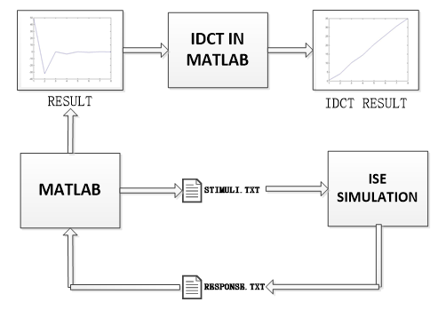
Figure 5, MATLAB ISE co-design procedure¶

Result ¶

The simulation result of the DCT can be shown in the APPENDIX 4 (a). As it shown in the figure, the result appears after two clock cycle. It is because of the pipeline of the whole system. This is called system latency. The speed improvement can’t be shown in this simulation because it is only a behavioral simulation, no delay is considered here. The input is (0, 5, 10, 15, 20, 25, 30, 35). In the MATLAB, this result can be plot as it shown in FIG6 .

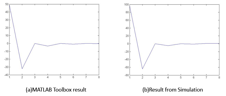
Figure 6, Simulation Result¶

As we can see in the result, there is a scale difference here. But the waveforms basically match with each other. There is some little difference in the results that is because of the round off in our hardware implementation. Since we didn’t implement the IDCT, I will use IDCT in MATLAB toolbox to transfer the cosine domain wave back to time domain to see the difference. The result can be shown in FIG7 .

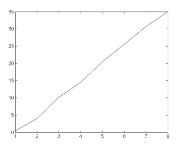
Figure 7, iDCT result in Matlab¶

Conclusion and Future Work ¶

In this project, we implement the Discrete Wavelet Transform using two different methods. One is DCT with algorithm reduction, one is binDCT using lifting block. The area of the binDCT is much smaller than the area in DCT. The Delay of the DCT is smaller than the delay of binDCT.

For the further work, we can design and implement the hardware of IDCT and using the IDCT to convert the cosine domain signal back to time domain. What is more, we can use the DCT implementation to realize the application of audio signal compression.

Reference ¶

[1] Jie Liang, Student Member, IEEE, and Trac D. Tran, Member, IEEE. Fast Multiplierless Approximations of the DCT With the Lifting Scheme1996

Statement

This is a course project, all the raw data are provided by Dr. Erdal Oruklu thought course ECE584 at IIT. Please contact me if you find any problem.