ECE587 Hardware/Software Codesign (Fall2013)¶

Introduction¶

This is the second project of the course ECE 587, the main purpose of this project is to build and evaluate a system that computes 8 point discrete Fourier transform (DFT) using fast Fourier transform which is known to us by FFT. FFT can efficiently transform a signal from time domain to the frequency domain, which will benefit the calculation of the response of a system or in some other areas. The FFT computation is based on the NoC architecture that we start in project #1. Instead of building a 1-D NoC architecture, we will build a 2-D NoC architecture to improve the efficiency of the computation. However, this system will be much more complex than the one in project #1. After building the NoC architecture, I am going to evaluate the system by printing some important parameters.

The whole project is based on the SystemC in a C++ environment. So the whole system is more like a simulation and this is very important to evaluate a system before going to implement it in the hardware. In the progress of coding in the Visual Studio, we will use GIT to manage the project and submit it at last.

Background Knowledge¶

The first thing that we have to describe is the fast Fourier transform (FFT). A fast Fourier transform (FFT) is an algorithm to compute the discrete Fourier transform (DFT) and its inverse. A Fourier transform converts time (or space) to frequency and vice versa. Although FFT is a simplification of the Fourier transform, it also needs a lot of computation. So for simplicity, we will only consider an 8-point DFT in our project.

The inputs of the computation are 8 complex numbers x(0), x(1),…,x(7) and the outputs are the other 8 complex numbers X (0); X (1); : : : ; X (7). The mathematical relation is shown as follows,

\(X(k)=\sum_{n=0}^{7} x(n) \omega^{k n} \quad \mathrm{k}=0,1,2, \ldots, 7\)

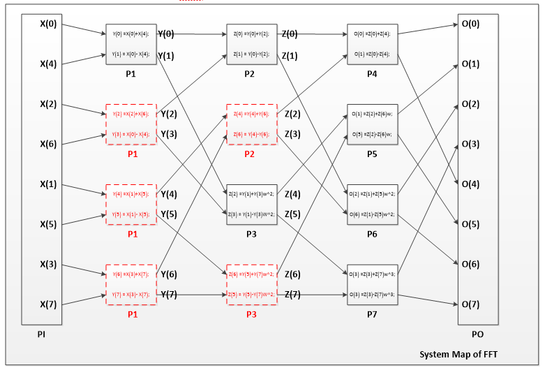
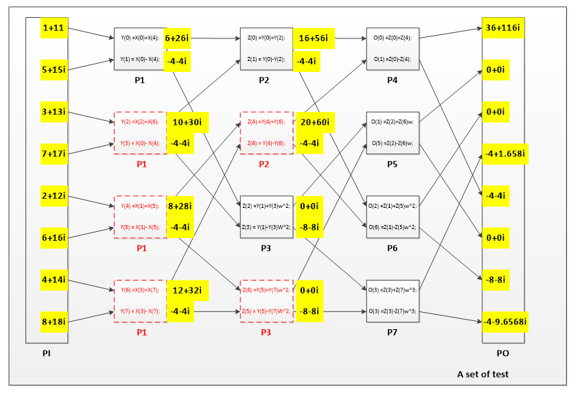
Where ω= ⅇ^(-j π/4) =cosπ/4 – j sinπ/4. Obviously, this equation includes a lot of computation in it. The FFT algorithm computes the same output in a much smarter way that requires much less computations. Though the FFT algorithm is inevitably complicated for general cases, for our problem setting, it can be written as the following 12 sets of equations, each representing a butterfly computation that input and output 2 complex numbers.

y(0) = x(0) + x(4);	y (1) = x(0) - x(4);	1
y(2) = x(2) + x(6);	y (3) = x(2) - x(6);	2
y(4) = x(1) + x(5);	y (5) = x(1) - x(5);	3
y(6) = x(3) + x(7);	y (7) = x(3) - x(7);	4
z(0) = y(0) + y(2);	z (1) = y(0) - y(2);	5
z(2) = y(1) + y(3)w^2;	z (3) = y(1) - y(3)w^2;	6
z(4) = y(4) + y(6);	z (5) = y(4) - y(6);	7
z(6) = y(5) + y(7)w^2;	z (7) = y(5) - y(7)w^2;	8
X (0) = z(0) + z (4);	X (4) = z (0) - z (4);	9
X (1) = z(2) + z (6)w;	X (5) = z (2) - z (6)w;	10
X (2) = z(1) + z (5)w^2;	X (6) = z (1) - z (5)w^2;	11
X (3) = z(3) + z (7)w^3;	X (7) = z (3) - z (7)w^3;	12

So, our problem become how to map these equations into our 2-D NoC system.

2D NoC Architecture¶

Different from project #1, we will build a 2-D NoC architecture this time. So there are more things to consider of, like how to build the mesh, how to route the packets and so on. Let’s discuss it one by one.

In project #1, I have already described the specific content of the routers and pes. So I will directly skip that part and come to the building of the 2-D NoC architecture part. The NoC system is built up by some basic blocks, each block consist a router and a PE. The routers take charge of routing the packets and the PEs process the data in the packets.

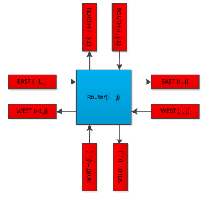
On the left side is a router. It has four directions, and each direction has to ports, one is input and one is output. The blue part is the router itself, and the red block is the data path. A data path can be regarded as a stack. One router push the packet into the stack and another one pop it. First in First out, acting like a FIFO. By connecting several routers like this, we can get a 2-D router mesh. As for the routers at the end of the mesh, we connect the output port to the input port of itself. This loop can improve the system robustness.

In the following picture is the system architecture of our design. It contains 9 routers and each router connects to a PE of its own. The PEs are represented in the red color and the routers are represented by blue blocks. I marked every data path with its name and the serial number. I assign PE(0, 0) as PI and PE(2, 0) as PO. PI is for generate the input for the whole system and also takes charge of printing the input data to the screen. PO takes charge of receiving the processed data from the whole system and printing it on the screen. Other PEs take charge of processing the data and routing the output data to next router after performing the equations to their inputs.

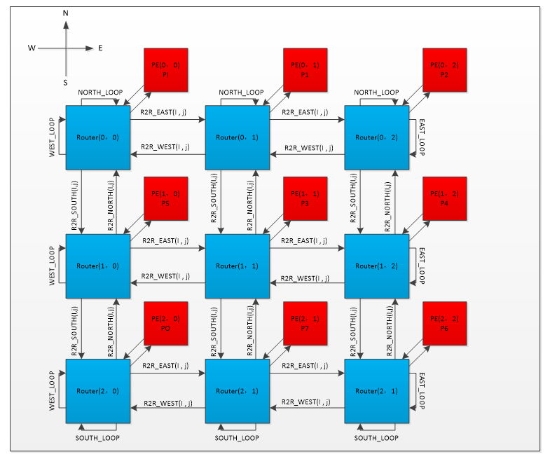
The following figure shows the way I map the pes to the routers. As you can find in the picture, the PEs are not mapped as the coordinate of itself. This is for the efficiency of the system. Take an example, PI will send the data directly to P1 at every cycle. There is no reason to separate PI and p1. For the same reason, I mapped the PEs as what it is shown in the picture. Although I didn’t make it to put every send and receive data pairs together, it is still a better way than mapping them in order.

System Implementation¶

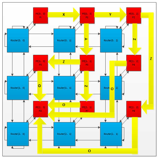
After connecting the routers and pes as a network, we are going to implement the FFT computation based on this 3*3 NoC architecture. The system is shown in the following picture.

There are basically three types of pes in the system. They are PI, PO and intermediate PE. For simplicity, I use just one kind of intermediate PE in the system. The tricky in this is I set every intermediate PE to the same function. Which means every PE contains all the equations. But every PE will only perform one kind of equations in the system. There are only 9 PEs in the 3*3 NoC system, so the red PEs don’t really exist. For example, after P1 process the data of X(0) and X(4), it will shift to the second place and process X(2) and X(6). In this way, we can map the whole system into 9 PEs.

In my system, the PI will stop sending data to P1 after it sends 8 complex numbers. It wait until the PO receive all the data and print it on the screen. Although it will badly decrease the throughput of the system. But this is the best way to avoid data violation.

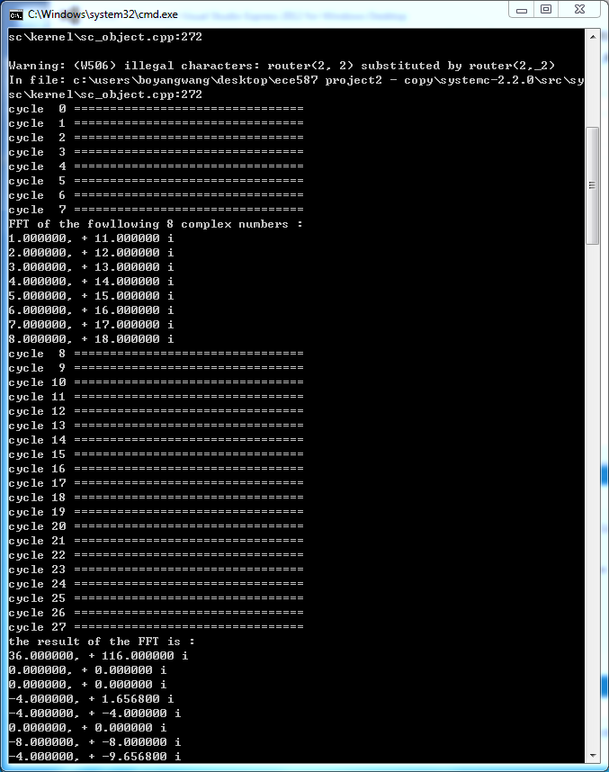
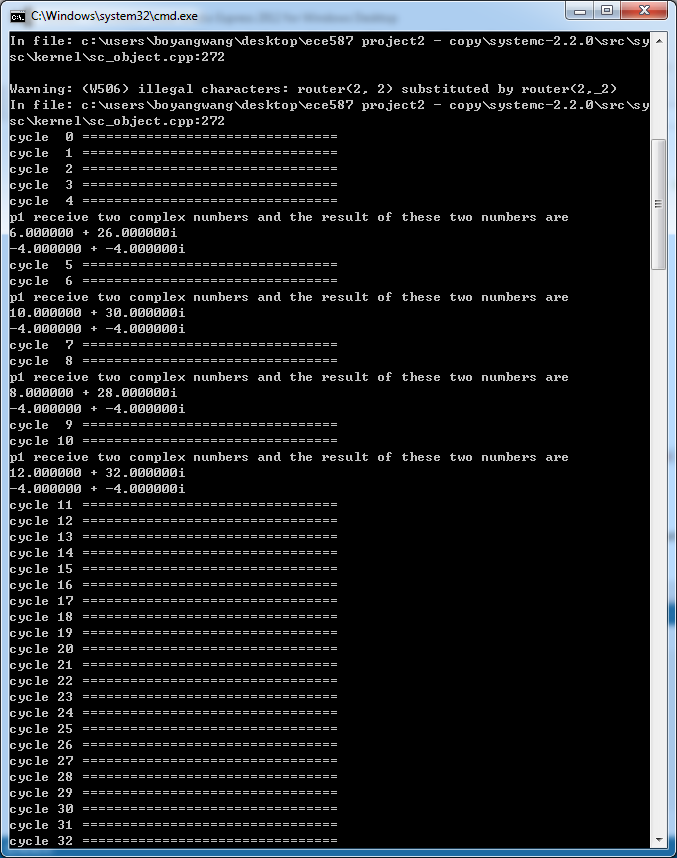
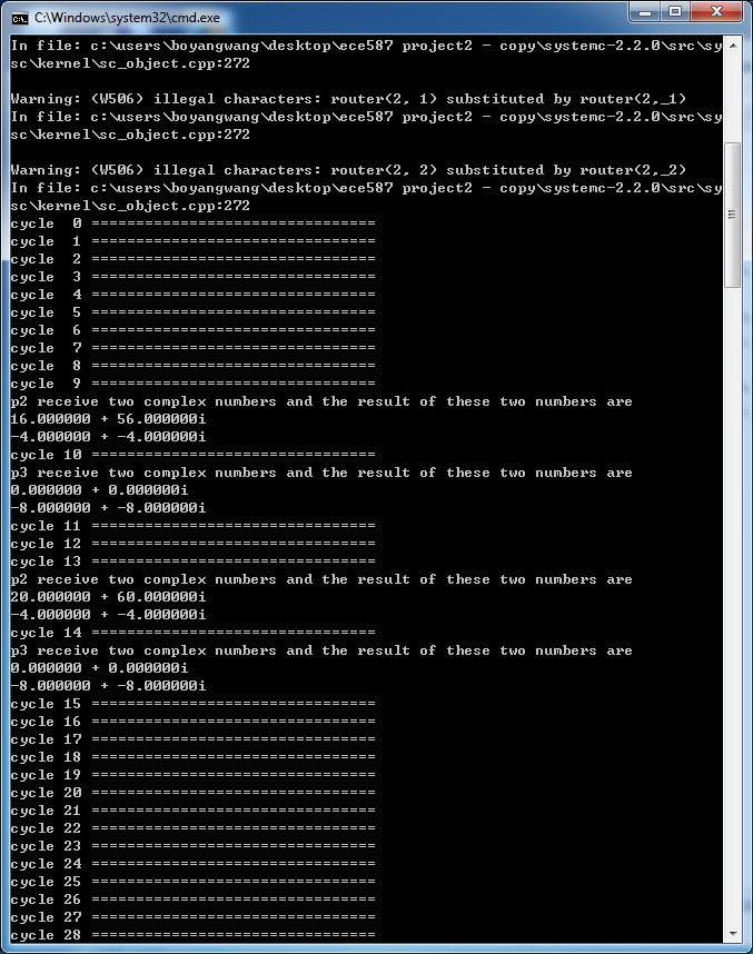
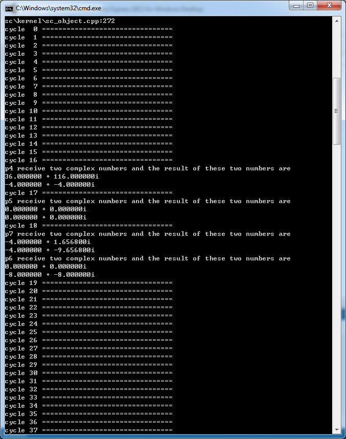
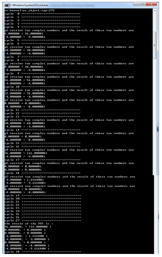
After I finish the system, I test the system with one group of complex numbers. An the result is shown in the following picture. The data flows in the NoC system, I give every equation an addition function of print the output after they performing the computation. By testing them one by one, I get the result of every node in the system. The result is exactly the same as the result that I calculated by my own.

System Evaluation¶

The most important performance metric is the maximum throughput. The maximum throughput is the sum of the data rates that are delivered to all terminals in a network. Since the packets is created by PI and consumed by P1 at first step. So the bottleneck of the system is when PI send data to P1. As it said in the project requirement, every PE can only generate 1 token and consume 1 token at 1 cycle. So generate one set of input at least will take 8 cycles. So the maximum throughput of the system is 1/8.

As for the computation latency, after we input the 8 complex numbers into the system, the cycles it will take to generate the output is the computation latency. We are supposed to measure the minimum latency. The minimum latency can be measured when there is only one set of inputs being processed in the NoC architecture. So I am going to check the first set of test to measure the minimum latency. The result is shown in the appendix. At the first cycle, the PI start to send the data to P1 and after 8 cycles, all 8 data are sent to the system and PI print the data on the screen. After another 20 cycles, PO receives all the data and prints it on the screen. The minimum latency of the system is 28 cycles.

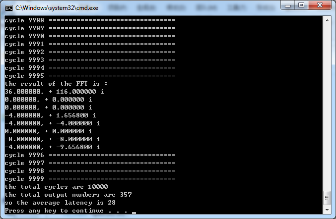
Then I am supposed to calculate the average numbers of the clock cycles needed to obtain outputs from the corresponding inputs. I set the clock cycles to 10000 and run it again. I use a counter in the PO, every time it print the data on the screen, I add the counter with one. Then I divide 10000 with the counter. I put the picture of the result in the appendix. The average latency of the system is 28. The average latency of my system is exactly the same as my minimum latency, that is because in all the time, there is only one set of data running in the system since I set the PI stop sending data until PO receive all the data.

Conclusion¶

This project is much more complex than the first one. If the first one is to let me get familiar with the NoC network, then this project is to tell me the practical usage of the NoC network. By connecting the microprocessors together with routers, we can realize some amazing functions. The FFT that we implement this time is just the tip of the submerged iceberg. There are more interesting and challenging things in this area that need us to develop. In the way that I built the system, there is one important thing is how to size the system. I can use just one piece of microprocessors to process the whole FFT computation, but it will take much more time than our system. This is quite a trade-off, we can use time to trade the hardware size, and we can also use more hardware to trade the time. It is very important when we design a system.