SidePrj: Split Spectrum Processing Implementation with Python (2018)

Introduction

This project serves as one of the components of my research project: Ultrasonic NDT Signal Acquisition and Processing System based on ZYNQ APSoC. Split Spectrum Processing is one of the very useful Time-Frequency Analysis techinques. We use this method for ultrasonic target echo detection. This page shows a python implementation of SSP using numpy, scipy, and matplotlib Python libraries. The SSP processing algorithm is very clearly described in this page, we will not repeat that.

Implementation

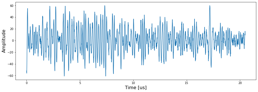
Load the original Signal into the workspace. The ultrasonic backscattered signal used in this post is sampled at 100 MSPS. We use following code to convert the time domain backscattered echoes into its frequency domain using np.fft.rfft from numpy

#convert all the data to frequency domain using rfft algorithm in numpy
rfftout = np.zeros((AllEchoData.shape[0],1025),dtype=complex)
for n in tqdm_notebook(range(AllEchoData.shape[0])):
    buf = np.fft.rfft(AllEchoData[n,:])
    buf.real[0] = 0 # remove the DC component
    rfftout[n,:] = buf

Figure 1. is the time domain ultrasonic backscattered signal and its FFT result.

Figure 1. Ultrasonic backscattered echo in time domain and frequency domain.

Next, we generate the Gaussian masks kernel_matrix with the following code:

#Generate Gaussian masks, with the following configurations
gaussianstep = 3
startfreq = 1e6
sigma = 3e5
endfreq = 10.3e6

listofmu = []
freq_axis = np.linspace(0,50e6,1025)
for items in freq_axis:
if items>=startfreq and items<endfreq:
    listofmu.append(items)
listofmu = listofmu[0::gaussianstep]
listlen = len(listofmu)

kernel_matrix = np.zeros((1025,listlen))
for i in range(listlen):
    kernel_matrix[:,i] = gaussian(freq_axis,listofmu[i],sigma)

Figure 2. demonstrates the Gaussian masks overlapped on the signal in frequency domain. In this demonstration case, the step is intentionally set to very small.

Figure 2. Generated Gaussian masks.

The SSP result sspresult can be acquired by converted the masked signals from its frequency domain back to time domain with:

maskedresult = kernel_matrix.transpose()*signal
maskedresult = maskedresult.transpose()
sspresult = np.zeros((2048,maskedresult.shape[1]))
for i in range(maskedresult.shape[1]):
    sspresult[:,i] = np.fft.irfft(maskedresult[:,i])

Results

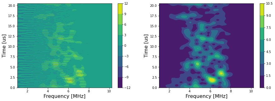
The result and its envelope can be plotted with contourf in matplotlib:

Fs = 100 #MHz
T = 1/Fs #us
N = 2048
t = T*N
time_axis = np.linspace(0,t,N)

plt.figure(figsize=(15,5))
plt.subplot(1,2,1)
frequencylist = np.asarray(listofmu)
_ = plt.contourf(frequencylist/1e6,time_axis,sspresult)
_ = plt.xlabel('Frequency [MHz]', fontsize=16)
_ = plt.ylabel('Time [us]', fontsize=16)
_ = plt.colorbar()

# acquire the envelope using Hilbert transform
plt.subplot(1,2,2)
sspresultenvlope = np.zeros((2048,maskedresult.shape[1]))
for i in range(maskedresult.shape[1]):
    hilbert = signal.hilbert(sspresult[:,i])
    sspresultenvlope[:,i] = np.abs(hilbert)

_ = plt.contourf(frequencylist/1e6,time_axis,sspresultenvlope)
_ = plt.xlabel('Frequency [MHz]', fontsize=16)
_ = plt.ylabel('Time [us]', fontsize=16)
_ = plt.colorbar()
plt.show()

Figure 3. is the contourf plots of SSP result and its envelope.

Figure 3. SSP result and its envelope plotted using contourf.

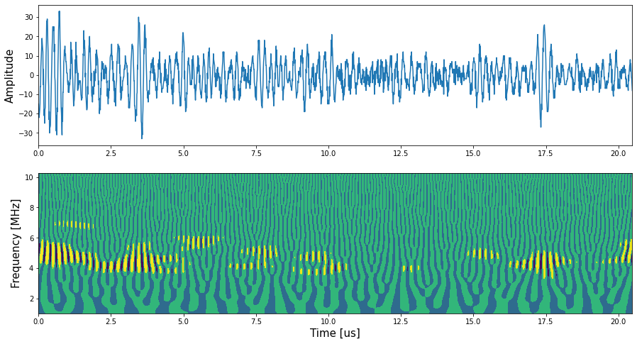
Figure 4. is the ultrasonic backscatered echo plotted against its SSP result.

Figure 4. Ultrasonic backscattered echo plotted againts the SSP result.